Bayesian Networks
Probability Basics
Before going into the details of Bayesian Network, let us revise the basics of probability. For event $A$ and $B$,
- $0 \leq \Pr(A) \leq 1$,
- $\Pr(A \cup B)=\Pr(A)+\Pr(B)-\Pr(A \cap B)$,
- $\Pr(True)=\Pr(U)=1$ where $U$ is the universal set,
- $\Pr(False)=\Pr(\phi)=0$ where $\phi$ is the empty set.
Independence: Events $A$ and $B$ are independent if $\Pr(A|B)=\Pr(A)$
Conditional Independence: Given event $B$, event $A$ is conditionally independent of event $C$ if $\Pr(A|B \cap C)=\Pr(A|B)$.
Additionally, we define the joint probability of events $A$ and $B$ as $\Pr(A,B)\equiv \Pr(A\cap B)$.
Bayes’ Rule: The conditional probability of event $A$ given event $B$ is computed based on their joint and independent probability using the following formula.
\[\Pr(A|B)=\frac{\Pr(A \cap B)}{\Pr(B)}\]By extension,
\[\Pr(A \cap B)=\Pr(B)\cdot \Pr(A|B)\] \[\Pr(A|B)=\frac{\Pr(A \cap B)}{\Pr(B)}=\frac{\Pr(A)\cdot \Pr(B|A)}{\Pr(B)}\]Law of Total Probability states that if $B_1, B_2, B_3, \cdots $ serve as a partition of the sample space $S$, then for any event $A$, we have
\[\Pr(A)=\sum \limits_i \Pr(A \cap B_i)= \sum \limits_i \Pr(A|B_i)\cdot \Pr(B_i)\]Probability in Partially Observable Environments
Suppose there are two coins in a jar: $C_{50}$ and $C_{90}$. The subscripts for each of the coin represents the bias of the coin.
Coin $C_{50}$ where the probability of heads given that the coin is flipped is $\Pr(H| C_{50})=50\%$
Coin $C_{90}$ where the probability of heads given that the coin is flipped is $\Pr(H|C_{90})=90\%$
A man walks to the jar, picks a coin from the jar and tosses the coin repeatedly 6 times. The goal of the agent is to make an educated guess of which coin the man had picked. The agent is unable to identify whether the coin is $C_{50}$ or $C_{90}$ through its sensors; however, he/she is able to observe the results for each of the man’s toss.
Prior to the toss, with no further information, it is equally likely to the agent that either coin be picked. Thus, the unconditional probability of the man picking $C_{50}$ or $C_{90}$ are $50\%$. However, with the information observed from the man’s repeated tosss of the coin, a more accurate judgment can be made. Let consider that the agent observed the following results of all 6 coin tosses $\langle HTTHTH \rangle$. The agent can use Bayes’ rule to update the probability estimates of the coin being $C_{50}$ or $C_{90}$ conditioned on this new information. At this point, the agent needs to models its beliefs.
| Before Toss | After Toss |
|---|---|
| $\Pr(C_{50}) = 0.5$ | $\Pr(C_{50}|\text{Toss})=?$ |
| $\Pr(C_{90}) = 0.5$ | $\Pr(C_{90}|\text{Toss})=?$ |
To calculate $\Pr(C_{50}|\text{Toss})$ and $\Pr(C_{90}|\text{Toss})$, we can use Bayes’s rule and law of total probability. By applying these two rules, we get $\Pr(C_{50}| \text{Toss}) > \Pr(C_{90}|\text{Toss}).$
\[\begin{aligned} \Pr(C_{50}|\text{Toss}) & = \dfrac{\Pr(C_{50} \cap \text{Toss})}{\Pr(\text{Toss})}\\ & = \dfrac{\Pr(\text{Toss}|C_{50}). \Pr(C_{50})}{\Pr(\text{Toss})}\\ & = \dfrac{0.5 \times (0.5)^6}{0.5 \times (0.5)^6 + 0.5 \times (0.9)^3 (0.1)^3}\\ & = 0.95 \end{aligned}\] \[\begin{aligned} \Pr(C_{90}| \text{Toss}) & = \dfrac{\Pr(C_{90} \cap \text{Toss})}{\Pr(\text{Toss})}\\ & = \dfrac{\Pr(\text{Toss}|C_{90}). \Pr(C_{90})}{\Pr(\text{Toss})}\\ & = \dfrac{0.5 \times 0.9^3 \times 0.1^3}{0.5 \times (0.5)^6 + 0.5 \times (0.9)^3 (0.1)^3}\\ & = 0.04 \end{aligned}\]The method of updating the agent’s beliefs on the probability of outcomes is summaries by Figure 1, where initially there are two contending models: $M_1:$ Coin $C_{50}$ is chosen and $M_2:$ Coin $C_{90}$ is chosen. Through some partial observations of the coin toss, the agent is able to use conditional probabilities to determine which model to chose.
 |
|---|
| Figure 1: Model classification with conditional probabilities |
In fact, this can be generalized to a case of $n$ coins. However, as $n$ grows large, it can be increasingly cumbersome to compute the conditional probabilities. For example, let’s consider the case of having 100 coin $C_1,C_2,C_3, \cdots , C_{100}$ where the subscripts indicate the percentage point probabilities of each coin landing a heads when tossed. Suppose you observe $k$ tosses, denoted $Toss$. Then the following probabilities have to be computed.
\[\begin{aligned} \Pr(C_1|Toss)&=\frac{\Pr(C_1)\Pr(Toss|C_1)}{\Pr(Toss)} \\ \vdots \\ \Pr(C_{100}|Toss)&=\frac{\Pr(C_{100})\Pr(Toss|C_{100})}{\Pr(Toss)} \\\end{aligned}\]where each $\Pr(Toss)$ is computed as,
\[\Pr(Toss)=\sum \limits_{i=1}^{100} \frac{1}{100} \Pr(Toss|C_i)\]Computing $\Pr(Toss)$ is cumbersome and also unnecessary for the agent to find which coin is most likely to be picked. Since the denominator in conditional probability of $\Pr(C_i|Toss)$ have the same $\Pr(Toss)$ for all the coins $C_i$, we only need to compute the numerator for comparison. In other-words,$\forall i,j$
\[\Pr(C_i|Toss)>\Pr(C_j|Toss) \Leftrightarrow \Pr(C_i)\Pr(Toss|C_i)>\Pr(C_j)\Pr(Toss|C_j)\]Thus, we only need to find the coin with the highest $\Pr(C_i)\Pr(Toss|C_i)$ values for that coin to be most likely to be picked.
Now, the important question is how to store this conditional probabilities and use them in an efficient manner to chose a model.
Consider a situation where a researcher is interested in predicting how likely a graduate student performs well in a job interview. Some factors to consider could be the graduate’s grades or even whether the graduate has to pay a road toll (ESP: Electronic Surge Pricing) on the way to the interview.
Events that have to be tracked are as follows.
Grades ($G$), where $G$ means that the graduate’s grades are high, and $\bar{G}$ means the graduate’s grades are low.
Having to pay Electronic Surge Pricing ($E$) where $E$ means that a graduate has been charged for ESP, and $\bar{E}$ means the graduate was not charged.
Job Interview ($I$), where $I$ means that the graduate’s interview goes well, and $\bar{I}$ means the graduate’s interview goes awry.
Let’s assume that the researcher had collected data from a sample of 600 students, and the joint frequency for every combination of $G$, $E$ and $I$ had been tallied. A naive way to store the values will be a simple table as shown below.
| $G$ | $E$ | $I$ | Frequency | $\Pr(C,G,I)$ |
|---|---|---|---|---|
| T | T | T | 160 | 160/600 |
| T | T | F | 60 | 60/600 |
| T | F | T | 240 | 240/600 |
| T | F | F | 40 | 40/600 |
| F | T | T | 10 | 10/600 |
| F | T | F | 60 | 60/100 |
| F | F | T | 10 | 10/600 |
| F | F | F | 20 | 20/600 |
Table 1: The tabulated joint probabilities for combination of events.
From the above table, we can compute both conditional and unconditional probabilities. For example, the probability of $\Pr(G)$ is the sum of all the joint probabilities in the table where the value of $G$ is true (T).
\[\begin{aligned} \Pr(G)&=\Pr(G,E,I)+\Pr(G,E,\bar{I})+\Pr(G,\bar{E},I)+\Pr(G,\bar{E},\bar{I}) \\ &=\frac{160+60+240+40}{600} \\ &=\frac{500}{600}\end{aligned}\]Similarly, the conditional probability of $G$ given $E$ can be computed as the sum of the joint probabilities of where both $G$ and $E$ in the row are true divided by the sum of joint probabilities where $E$ is true.
\[\begin{aligned} \Pr(G|E)&=\frac{\Pr(G\cap E)}{\Pr(E)} \\ &=\frac{\Pr(G,E,I)+\Pr(G,E,\bar{I})}{\Pr(G,E,I)+\Pr(G,E,\bar{I})+\Pr(\bar{G},E,I)+\Pr(\bar{G},E,\bar{I})} \\ &=\frac{160+60}{160+60+10+60} \\ &=\frac{220}{290}\end{aligned}\]Space and Computational Complexity
One major drawback in the tabular form is that the tables can be huge when there are more variables. This means that the method of storing the joint probabilities in a tabular form is not scalable to larger problems. If there are 5 variables, then there will need to be $2^5=32$ entries. However, to be precise, as the sum of probabilities is 1, we can exclude the last entry (and compute it by subtracting all the other probabilities from 1).
In particular, if there are $n$ variables with two values (true or false), then the space and computational complexity is $\mathcal{O}(2^n)$.
Representing Information as Directed Acyclic Graph: Bayesian network
Suppose there are 5 variables:
- Grades(G)
- ESP(E)
- Interview (I)
- Job Offer (J)
- Driver’s Mood(D)
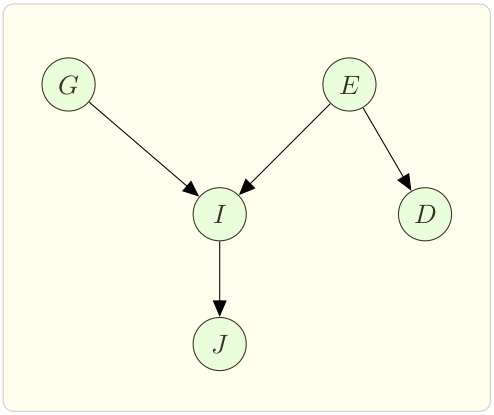
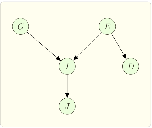
We can represent the causal information of these variables in the form of a Directed Acyclic Graph (DAG). For example, we know that Grades and having to pay ESP are causal factors of Interview performance. Interview performance in turn directly affects the Job offer. However, we know that having to pay ESP can causally affects the Driver’s mood, but the Driver’s mood cannot causally affect any other variable. With that we form the graph as shown in Figure 2.
 |
|---|
| Figure 2: Bayesian Network |
In Figure 2, each variable is represented by a node. The causal relation is represented by a directed edge from one variable to another. The network captures how well the interview goes based on grades and ESP.
Next, we want to store the conditional probabilities associated with each node in the form of a table. Bayesian Network Law says, given parents, the probability of a node is independent of its non-descendants, i.e. each node in a Bayesian network is independent of all non-descendants node, given its parents. As in Figure 2, $\Pr(I|G,E,D) = \Pr(I|G,E)$.
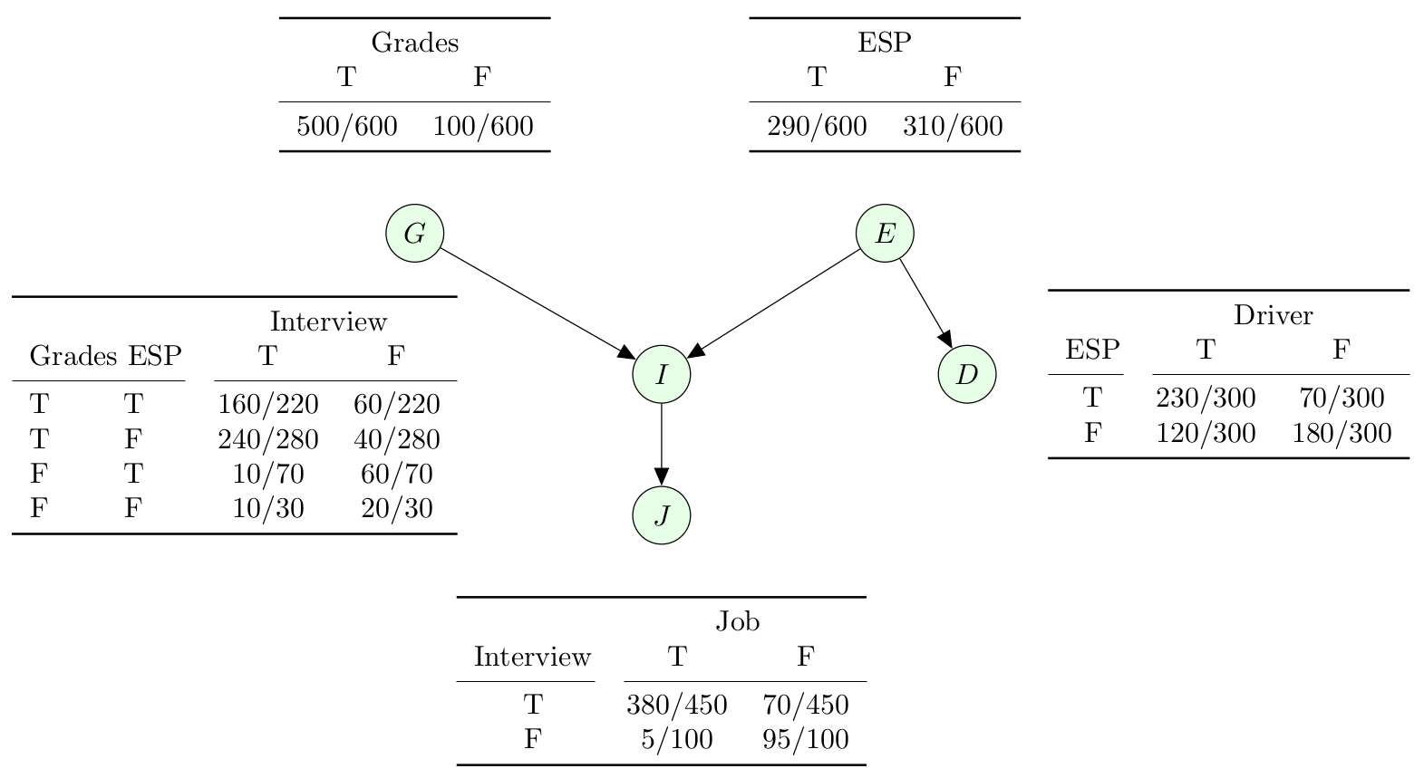
Figure 3 represents a Bayesian Network or an Inference Network. Each table of Figure 3 is called a conditional probability table (CPT). For tables associated with nodes such as Grades, ESP with no causal factor, the conditional probability of those nodes is the same as their unconditional probability.
 |
|---|
| Figure 3: Conditional Probability Table |
How did we come up CPT from Table 1?
We processed Table 1 in row by row manner to fill up CPTs.
| $G$ | $E$ | $I$ | Total | $\Pr(C,G,I)$ |
|---|---|---|---|---|
| $T$ | $T$ | $160$ | $160+60=220$ | $\frac{160}{220}$ |
| $T$ | $F$ | $240$ | $240+40=280$ | $\frac{240}{280}$ |
| $F$ | $T$ | $10$ | $10+60=70$ | $\frac{10}{70}$ |
| $F$ | $F$ | $10$ | $10+20=30$ | $\frac{10}{30}$ |
Space Complexity of Bayesian Network
As discussed earlier, tabular representation requires 32 entries for 5 variables. With Bayesian network representation, it requires 10 rows. Assuming that in the DAG, the maximum number of parents is a positive integer $q$, the number of entries required in the worst case is $n2^q$ in a Bayesian network. This makes the space complexity $\mathcal{O}(n2^q)$, which is an improvement from $2^n$.
Computing Probabilities in a Bayesian Network
Now that we have the network, we can compute the joint probabilities of multiple variables efficiently. We can use the chain rule formula to break the computation into a multiplication of a series of conditional probabilities.
The joint probability of events $X_1,X_2,\cdots ,X_n$ is the following,
\[\Pr(X_1,X_2,\cdots X_n)=\Pr(X_1|X_2, X_3, \cdots X_n) \Pr(X_2|X_3, X_4, \cdots X_n) \cdots \Pr(X_{n-1}|X_n)\Pr(X_n)\]In our example, one way to compute the joint probability of $G,I,J,E,D$ is,
\[\begin{aligned} \Pr(G,I,J,E,D)=\Pr(G|I,J,E,D)\cdot \Pr(I|J,E,D) \cdot \Pr(J|E,D) \cdot \Pr(E|D) \cdot \Pr(D)\end{aligned}\]However, we encounter a problem with this particular order in the chain rule. None of the conditional probabilities in the expression above are readily extractable from the Bayesian Network. Instead, we can reorder the variables and apply the chain rule in a specific order that allows us to extract the conditional probabilities from the Bayesian network. One way to find such an order is to first pick a variable that has no children, remove the node and repeat. Since Bayesian network is a DAG, there must exists at least one node with no children. One such ordering for the example in Figure 2 is $J,I,G,D,E$.
\[\begin{aligned} \Pr(G,I,J,E,D)&=\Pr(J,I,G,D,E) \\ &=\Pr(J|I,G,D,E)\cdot \Pr(I|G,D,E)\cdot \Pr(G|D,E)\cdot \Pr(D|E)\cdot \Pr(E) \\ &=\Pr(J|I)\cdot \Pr(I|G,E) \cdot \Pr(G) \cdot \Pr(D|E) \cdot \Pr(E) \end{aligned}\]d-separation: Determining Independence of Variables
Now the question becomes, how do we determine if two variables $X$, $Y$ are independent given a given set of variables $E$? There is a simple graphical property called d-separation to solve this question that works in the following way
- A set of variables $E$ d-separates $X$ and $Y$ if it blocks every undirected path in the BN between $X$ and $Y$. (We’ll define blocks next.)
- $X$ and $Y$ are conditionally independent given evidence $E$ if $E$ d-separates $X$ and $Y$.
- thus BN gives us an easy way to tell if two variables are independent (set $E = \emptyset$) or cond. independent given $E$.
Blocking in d-Separation
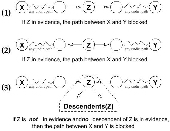
Let $P$ be an undirected path from $X$ to $Y$ in a BN. Let $E$ (evidence) be a set of variables. We say $E$ blocks path $P$ iff there is some node $Z$ on the path $P$ such that any of the following cases hold:
- Case 1: $Z\in E$ and one arc on $P$ enters (goes into) $Z$ and one leaves (goes out of) $Z$.
- Case 2: $Z\in E$ and both arcs on $P$ leave $Z$.
- Case 3: both arcs on $P$ enter $Z$ and neither $Z$, nor any of its descendents, are in $E$.
In Figure 4, we show d-separation in a graphical view.
 |
|---|
| Figure 4: Blocking in d-separation |
Deciding the Optimal Model
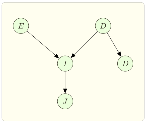
Suppose we are given two different models of Bayesian network and an evidence. Now the question is which of the Bayesian network would we choose? For example, instead of believing that Driver’s mood depends on ESP, we may believe that Driver’s mood depends on Student’s grades. Now, as shown in Figure 5, we have 2 Bayesian networks. Also, we have 2 evidences:
$e_1 :G = T, E = T, D = F, I = T, J = F$
$e_2 : G = T, E = F, D = T, I = T, J = F$
 |  |
|---|---|
| Bayesian Network M1 | Bayesian Network M2 |
Figure 5: Two Bayesian Networks.
We want to decide which of the two models is a more likely description of evidences $e_1$ and $e_2$. Thus we need to determine if
\[\begin{aligned} \Pr(M_1|\{e_1,e_2\}) & \overset{?}{\geq} \Pr(M_2|\{e_1,e_2\}) \\ \dfrac{\Pr(M_1|\{e_1,e_2\})}{ \Pr(M_2|\{e_1,e_2\})} & \overset{?}{\geq} 1. \end{aligned}\]We know that
\[\label{eq:1} \Pr(M_1|\{e_1,e_2\}) = \dfrac{\Pr(\{e_1,e_2\}|M_1) \times \Pr(M_1)} {\Pr(\{e_1,e_2\})},\] \[\label{eq:2} \Pr(M_2|\{e_1,e_2\}) = \dfrac{\Pr(\{e_1,e_2\}|M_2) \times \Pr(M_2)} {\Pr(\{e_1,e_2\})}.\]Since we are interested in computing the ratio of \({\Pr(M_1|\{e_1,e_2\})}\) and \({ \Pr(M_1|\{e_1,e_2\})}\), we don’t need to compute \({\Pr(\{e_1,e_2\})}\) as it is cancelled out in the ratio. We also assume that the data collected are independent of each other. Thus, \(\Pr(\{e_1,e_2\}|M_1)=\Pr(e_1|M_1)\Pr(e_2|M_1)\) and \(\Pr(\{e_1,e_2\}|M_2)=\Pr(e_1|M_2)\Pr(e_2|M_2)\). Finally, we require to compute $\Pr(M_1)$ and $\Pr(M_2)$, as discuessed next.
$\Pr(M_1)$ and $\Pr(M_2)$ reflect the probabilities of each of the models occurring in real life. In fact, it is often difficult to obtain these probabilities. There are several possible ways to compute these probabilities.
We may choose to start with prior distributions for $\Pr(M_1)$ and $\Pr(M_2)$ based on our own past experiences.
We may also compute the values of $\Pr(M_1)$ and $\Pr(M_2)$ on historical information from the usage of either of these models.
However, it is only necessary for us to compute the ratio $\Pr(M_1)/\Pr(M_2)$, since we compare the magnitude of \(\Pr(M_1|\{e_1,e_2\})\) with \(\Pr(M_2|\{e_1,e_2\})\).
How to come up with models $M_1$ and $M_2$
We can use any of the local search algorithms to find a good model to work with. In local search, we start with an arbitrary state and make a transition to another state depending on the value assigned to that state. For example, we can start with model $M_1$, where $M_2$ is its neighboring model. We make a transition from $M_1$ to $M_2$, if given an evidence $e_1$, $\Pr(M_1|{e_1}) < \Pr(M_2|{e_1})$.
Thus, the algorithm for obtaining an optimal model based on evidences is in the following:
Initialize a random model.
At every step, look for a neighbor $N(M)$ of the current model.
Compute $\tfrac{\Pr(\text{evidence}|N(M))}{\Pr(\text{evidence}|M)}$, where $N(M)$ is a neighbor of model $M$.
Make a transition to a new model only if ratio is greater than $1$, else terminate with model $M$.