Variable Elimination in Bayesian Networks

As discussed in last lecture, Bayesian Networks (BNs) are a class of graphical models that represent the conditional dependencies between a set of variables. They are way to model probability distributions, and used to model probabilistic relationships in complex systems, where the nodes represent variables and the edges signify the dependencies.

In this lecture, we’ll focus on efficiently computing joint probabilites of events given a network. We’ll learn a tool called variable elimination for that.

For that, we’ll use three tools that we already know:

1. Bayesian network law says, Given parents, a node is independent of its non-descendents.

2. D-separation is a technique used to determine if two variables in a BN are independent, given a set of other variables. It is based on the graphical structure of the network. A set of nodes $D$ is said to d-separate $X$ from $Y$ if it blocks every path from $X$ to $Y$. The criteria for D-separation is as follows:

   1. If a node is observed, it blocks the path.
   2. A path is blocked if it includes a chain or a fork with an observed node.
   3. A collider blocks the path if neither the collider nor its descendants are observed.

3. Chain rule says, ${\displaystyle \Pr (A, B)=\Pr (B\mid A)\Pr (A)}$

Practice Problem 1

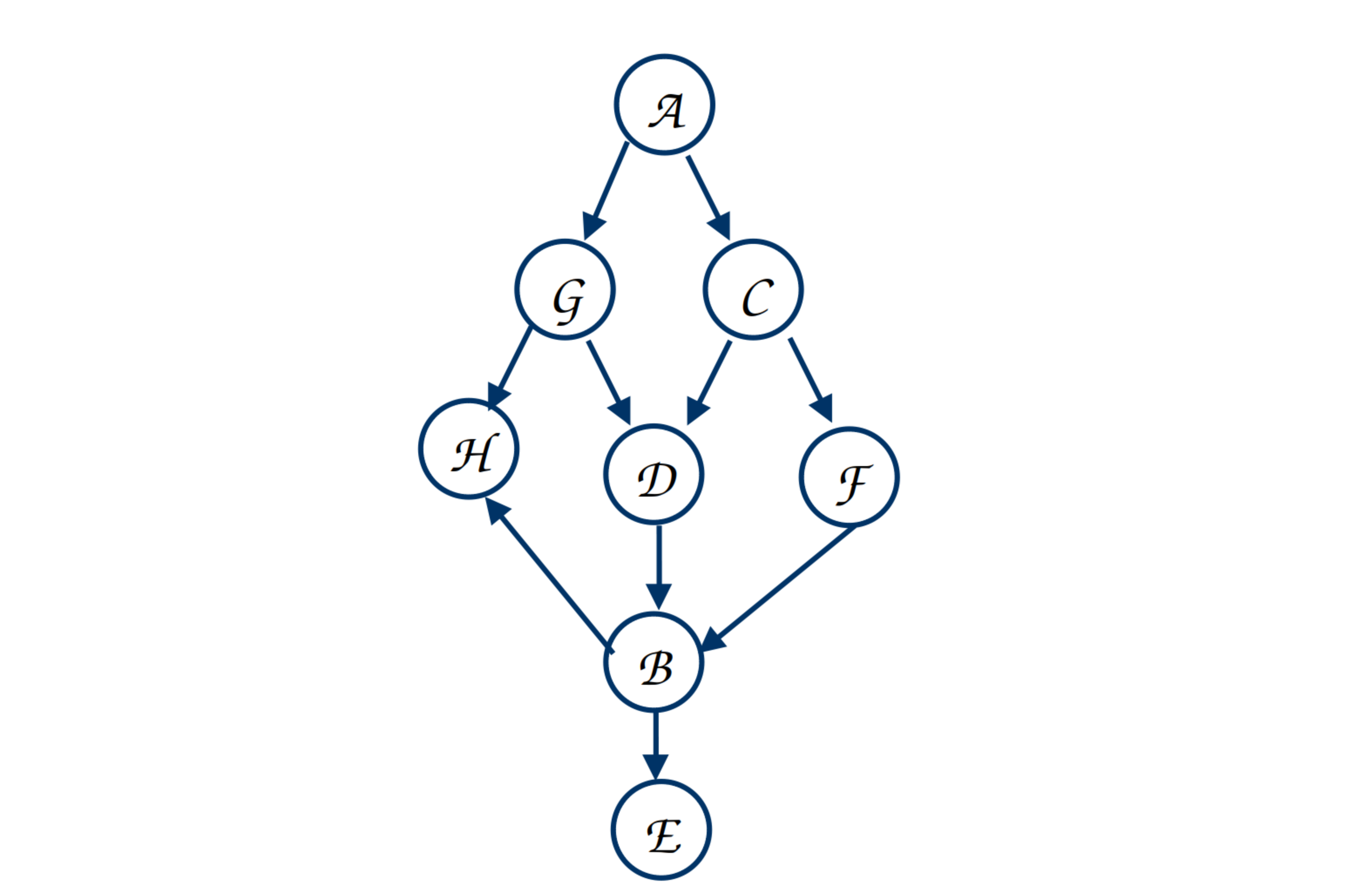
From network 1 in figure 1, Can we say, given G and C, whether E is independent of A? Approach: If we can show that $\Pr(E | A, G, C) = \Pr(E | G, C)$, then we can say that. Therefore, we’ll start by calculating $\Pr(E | A, G, C)$.

Figure 1: Example Bayesian Network 1

As $E$ has $B$ as its parent, to apply Bayesian network law we have to introduce $B$ into the equation, we do the following. We’ll use the notation $\displaystyle\sum_{A} \Pr(A)$ to denote the sum of probabilities over all the values that $A$ can take. Now, $D$ can take two values $d$ and $\neg d$. Therefore, $\displaystyle\sum_{A} \Pr(A) = \Pr(a) + \Pr(\neg a)$. \(\begin{align} \Pr(E | A, G, C) &= \sum_B \Pr(E, B | A, G, C) \end{align}\)

Using chain rule, we can say:

Now we can apply BN law - given $B$, $E$ is independent of $A,G,C$. Therefore,

To calculate $\Pr(B | A, G, C)$, to use BN law, again we are needed to introduce parents of $B$, i.e., $D,F$. Now,

Using chain rule, we get,

Now, given $D$ and $F$; $B$ is independent of $G,A,C$. Therefore, $\Pr(B|D,F, G,A,C) = \Pr(B|D,F)$. Similarly, $\Pr(D| G,A,C)= \Pr(D| G,C)$ and $ \Pr(F| G,A,C) = \Pr(F| C)$. Therefore, $\Pr(B,D,F | G,A,C) = \Pr(B,D,F | G,C)$.

Now, following equation 2, we get $\Pr(B | A, G, C) = \Pr(B | G, C) $. We can put this value to equation 2, then in equation 1 to finally show that $\Pr(E | A, G, C) = \Pr(E | G, C)$. Therefore, we can conclude that E is independent of A.

Computing Joint Probabilities

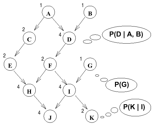
Now we want to compute the probability $\Pr(A,B,C,D,E,F,G,H,I,J,K)$ from network 2 in Figure 2.

Figure 2: Example Bayesian Network 2

From the network 2, we can write as following:

Problem:

Say that $E = \{H=true, I=false\}$, and we want to know $\Pr(D | h, \neg i)$

$~~~~~~~~~~~~~~~~~~~~~~~~(h$: $H$ is true, $\neg h$: $H$ is false$)$

So we are computing $\Pr(d, h, \neg i)$ and $\Pr(\neg d, h, \neg i)$ divided by their sum. Let’s focus on just computing $\Pr(d, h, \neg i)$ which equals

Using the network, we can rewrite this summation as:

We can definitely do the summation by taking all possible values for each of the variables, $A,B,C,\dots$, but the number of all possible combination for these 8 variables will be $2^8$, a value exponential of number of nodes of the network. The question becomes, can we do better somehow. For that, we’ll do three different steps.

Step 1: Rearranging Summations

The first step is to, rearrange summations so that we are not summing over variables that do not depend on the summed variable:

We can further rearrange the terms:

Step 2: Getting Constant Factors

Now start computing from the last summation to the first.

Now, $\displaystyle\sum_{A} \Pr(K | \neg i) = \Pr(k | \neg i) + \Pr(\neg k | \neg i) = c_1$. The value of $c_1$ does not depend on any of the variables so we can move it to the front. Now we have a new expression that does not have the variable $K$. $K$ has been eliminated and we have the following expression:

Similar to $K$, here $\sum_{J} \Pr(J | h, \neg i) = \Pr(j | h, \neg i) + \Pr(\neg j | h, \neg i) = c_2$, and we can eliminate $J$ and get the follwing expression:

Step 3: Introducing functions

Now, $\Pr(\neg i | F, g)$ depends on the value of $F$, so this is not a single number. So the sum depends on $F$. Once $F$ is fixed to $f$ or $\neg f$, the sum yields a fixed number. We introduce a function to represent this sum:

We can proceed by systematically eliminating variables one at a time until we sum over $A$, resulting in a singular value equivalent to $\Pr(d, h, \neg i)$. By executing a similar operation, we obtain $\Pr(\neg d, h, \neg i)$. Normalizing these two values yields $\Pr(d | h, i)$ and $\Pr(\neg d | h, i)$. Alternatively, we may retain $D$ as a variable and calculate a function of $D$, denoted as $f_k(D)$, which yields the desired outcomes through its two values $f_k(d)$ and $f_k(\neg d)$. This method is referred to as variable elimination. Through the computation of intermediate functions such as $f_1(F)$, $f_2(E)$, etc., we effectively store values for multiple uses throughout the computation. Thus, variable elimination serves as a dynamic programming technique, optimizing efficiency by preserving sub-computations to circumvent redundant calculations.

Generally, at each stage, elimination focuses on the innermost variable to compute a new function spanning the variables within that sum. This function assigns a specific number to each unique combination of its arguments. We archive these functions in a table, dedicating one entry to each variable instantiation. The magnitude of these tables grows exponentially with the number of variables involved in the sum, for example, contingent on the values of D and E. Consequently, the resultant table will encompass $|Dom[D]|*|Dom[E]|$ distinct values.